Quantum Espresso

The quantum espresso density-functional theory (DFT) simulation code is written in Fortran and uses the message passing interface (MPI) for parallelization, without any Python bindings. So executorlib is used to orchestrate multiple quantum espresso simulation each using multiple CPU cores for parallelization. These kind of hierarchical workflows are one of the core strength of executorlib. It is important to emphasize that the same could not be achieved with other frameworks like mpi4py as quantum espresso does not support external MPI communicators without modifications to the Fortran source code. With executorlib the user can quickly up-scale their simulation workflow without the need to address the parallel execution explicitly, rather the parallelization is introduced on a per-function level, by submitting the functions to the FluxClusterExecutor or FluxJobExecutor.

import os
import subprocess
from ase.build import bulk
from atomistics.workflows import (
    analyse_results_for_energy_volume_curve,
    get_tasks_for_energy_volume_curve,
)
import matplotlib.pyplot as plt
import pprint
from tqdm import tqdm
from time import sleep

The function which handles the parallel execution is the evaluate_with_quantum_espresso() function, internally it calls flux run pw.x to execute the quantum espresso Fortran executable in parallel:

def evaluate_with_quantum_espresso(task_dict, pseudopotentials, kpts):
    from ase.calculators.espresso import Espresso, EspressoProfile
    from atomistics.calculators import evaluate_with_ase
    
    return evaluate_with_ase(
        task_dict=task_dict,
        ase_calculator=Espresso(
            pseudopotentials=pseudopotentials,
            tstress=True,
            tprnfor=True,
            kpts=kpts,
            profile=EspressoProfile(
                 command="flux run pw.x",
                 pseudo_dir="/home/runner/work/executorlib/executorlib/tests/integration",
            ),
        ),
    )["energy"]

The pseudo potential is located in tests/integration, here the absolute path to the pseudo potential is given as: /home/runner/work/executorlib/executorlib/tests/integration.

pseudopotentials = {"Al": "Al.pbe-n-kjpaw_psl.1.0.0.UPF"}

As a first step of the workflow the equilibrium structure of four Aluminium atoms is strained by 5%.

task_dict = get_tasks_for_energy_volume_curve(
    structure=bulk("Al", a=4.15, cubic=True),
    num_points=7,
    vol_range=0.05,
    axes=("x", "y", "z"),
)

The resulting dictionary of structures task_dict is transformed to simplify the parallel execution:

task_loop_dict = {k: {"calc_energy": v} for k, v in task_dict["calc_energy"].items()}

The status of the flux cluster is validated using the flux resource list command and the flux jobs -a command, just to highlight flux was initialized correctly and has access to the available resources.

pprint.pp(subprocess.check_output(["flux", "resource", "list"], universal_newlines=True).split("\n"))

['     STATE NNODES   NCORES    NGPUS NODELIST',
 '      free      1        2        1 '
 'p200300e77f488c5f903797efb75a6bf7.dip0.t-ipconnect.de',
 ' allocated      0        0        0 ',
 '      down      0        0        0 ',
 '']

pprint.pp(subprocess.check_output(["flux", "jobs", "-a"], universal_newlines=True).split("\n"))

['       JOBID USER     NAME       ST NTASKS NNODES     TIME INFO', '']

FluxClusterExecutor

The FluxClusterExecutor is used in this demonstration primarily because flux can be installed on any workstation for testing. The SlurmClusterExecutor could be used analogously.

from executorlib import FluxClusterExecutor

The for each strained structure a calculation task is submitted to the FluxClusterExecutor. After the successful submission the current status of the flux queue is printed using flux jobs -a. Finally, the results are collected by gathering the concurrent.futures.Future objects.

future_dict = {}
with FluxClusterExecutor() as exe:
    for k, v in task_loop_dict.items():
        os.makedirs(os.path.abspath(("strain_%0.2f" % k).replace(".", "_")), exist_ok=True)
        future_dict[k] = exe.submit(
            evaluate_with_quantum_espresso, 
            task_dict=v, 
            pseudopotentials=pseudopotentials, 
            kpts=(3, 3, 3), 
            resource_dict={
                "cores": 1,  # As an external executable is used the number of cores is set to one
                "threads_per_core": 2,  # For external executables the number of threads_per_core specifies the parallel execution
                "cwd": os.path.abspath(("strain_%0.2f" % k).replace(".", "_")),
            },
        )
    sleep(1)
    pprint.pp(subprocess.check_output(["flux", "jobs", "-a"], universal_newlines=True).split("\n"))
    result_dict = {
        k: f.result() 
        for k, f in tqdm(future_dict.items())
    }
    sleep(1)
    pprint.pp(subprocess.check_output(["flux", "jobs", "-a"], universal_newlines=True).split("\n"))

['       JOBID USER     NAME       ST NTASKS NNODES     TIME INFO',
 '    ƒEmWEBP5 jan      2025-03-2+  S      2      -        - ',
 '    ƒErvXZ8B jan      2025-03-2+  S      2      -        - ',
 '    ƒEcB6hXD jan      2025-03-2+  R      2      1   0.846s '
 'p200300e77f488c5f903797efb75a6bf7.dip0.t-ipconnect.de',
 '']

100%|███████████████████████████████████████████████████████████████████████████████████████████████████████████████████████████████████████████████████████████████████████████████████████████████████████████| 7/7 [03:24<00:00, 29.15s/it]

['       JOBID USER     NAME       ST NTASKS NNODES     TIME INFO',
 '    ƒFSHFPtB jan      2025-03-2+ CD      2      1   9.355s '
 'p200300e77f488c5f903797efb75a6bf7.dip0.t-ipconnect.de',
 '    ƒFLoz3aP jan      2025-03-2+ CD      2      1   26.28s '
 'p200300e77f488c5f903797efb75a6bf7.dip0.t-ipconnect.de',
 '    ƒFF5tpT9 jan      2025-03-2+ CD      2      1   27.94s '
 'p200300e77f488c5f903797efb75a6bf7.dip0.t-ipconnect.de',
 '    ƒF2grpmu jan      2025-03-2+ CD      2      1    24.2s '
 'p200300e77f488c5f903797efb75a6bf7.dip0.t-ipconnect.de',
 '    ƒErvXZ8B jan      2025-03-2+ CD      2      1   43.07s '
 'p200300e77f488c5f903797efb75a6bf7.dip0.t-ipconnect.de',
 '    ƒEmWEBP5 jan      2025-03-2+ CD      2      1   28.25s '
 'p200300e77f488c5f903797efb75a6bf7.dip0.t-ipconnect.de',
 '    ƒEcB6hXD jan      2025-03-2+ CD      2      1   46.94s '
 'p200300e77f488c5f903797efb75a6bf7.dip0.t-ipconnect.de',
 '']

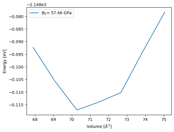
The resulting energies for the different volumes are fitted using a 3rd order polynomial to derive the bulk modulus as second derivative multiplied by the equilibrium volume.

fit_dict = analyse_results_for_energy_volume_curve(
    output_dict={"energy": result_dict},
    task_dict=task_dict,
    fit_type="polynomial",
    fit_order=3,
)

The final energy volume curve plot summarizes the results of this calculation.

plt.plot(fit_dict["volume"], fit_dict["energy"], label="$B_0$= %0.2f GPa" % fit_dict["bulkmodul_eq"])
plt.xlabel("Volume [$\AA^3$]")
plt.ylabel("Energy [eV]")
plt.legend()

<>:2: SyntaxWarning: invalid escape sequence '\A'
<>:2: SyntaxWarning: invalid escape sequence '\A'
/tmp/ipykernel_31059/4024930470.py:2: SyntaxWarning: invalid escape sequence '\A'
  plt.xlabel("Volume [$\AA^3$]")

<matplotlib.legend.Legend at 0x7f507c1bf020>

FluxJobExecutor

In analogy to the FluxClusterExecutor the FluxJobExecutor can be applied to distribute simulation within a given queuing system allocation. The calculation of the bulk modulus with quantum espresso is implemented in the same way.

from executorlib import FluxJobExecutor

The for each strained structure a calculation task is submitted to the FluxJobExecutor. After the successful submission the current status of the flux queue is printed using flux jobs -a. Finally, the results are collected by gathering the concurrent.futures.Future objects.

future_dict = {}
with FluxJobExecutor(flux_executor_nesting=True) as exe:
    for k, v in task_loop_dict.items():
        os.makedirs(os.path.abspath(("strain_%0.2f" % k).replace(".", "_")), exist_ok=True)
        future_dict[k] = exe.submit(
            evaluate_with_quantum_espresso, 
            task_dict=v, 
            pseudopotentials=pseudopotentials, 
            kpts=(3, 3, 3), 
            resource_dict={
                "cores": 1,  # As an external executable is used the number of cores is set to one
                "threads_per_core": 2,  # For external executables the number of threads_per_core specifies the parallel execution
                "cwd": os.path.abspath(("strain_%0.2f" % k).replace(".", "_")),
            },
        )
    sleep(1)
    pprint.pp(subprocess.check_output(["flux", "jobs", "-a"], universal_newlines=True).split("\n"))
    result_dict = {
        k: f.result() 
        for k, f in tqdm(future_dict.items())
    }
    sleep(1)
    pprint.pp(subprocess.check_output(["flux", "jobs", "-a"], universal_newlines=True).split("\n"))

['       JOBID USER     NAME       ST NTASKS NNODES     TIME INFO',
 '   ƒ2onx4eSU jan      flux        S      1      -        - ',
 '   ƒ2onyYdio jan      flux        S      1      -        - ',
 '   ƒ2onyYdip jan      flux        S      1      -        - ',
 '   ƒ2oo12d19 jan      flux        S      1      -        - ',
 '   ƒ2oo12d1A jan      flux        S      1      -        - ',
 '   ƒ2oo12d1B jan      flux        S      1      -        - ',
 '   ƒ2onx4eST jan      flux        R      1      1   0.994s '
 'p200300e77f488c5f903797efb75a6bf7.dip0.t-ipconnect.de',
 '    ƒFSHFPtB jan      2025-03-2+ CD      2      1   9.355s '
 'p200300e77f488c5f903797efb75a6bf7.dip0.t-ipconnect.de',
 '    ƒFLoz3aP jan      2025-03-2+ CD      2      1   26.28s '
 'p200300e77f488c5f903797efb75a6bf7.dip0.t-ipconnect.de',
 '    ƒFF5tpT9 jan      2025-03-2+ CD      2      1   27.94s '
 'p200300e77f488c5f903797efb75a6bf7.dip0.t-ipconnect.de',
 '    ƒF2grpmu jan      2025-03-2+ CD      2      1    24.2s '
 'p200300e77f488c5f903797efb75a6bf7.dip0.t-ipconnect.de',
 '    ƒErvXZ8B jan      2025-03-2+ CD      2      1   43.07s '
 'p200300e77f488c5f903797efb75a6bf7.dip0.t-ipconnect.de',
 '    ƒEmWEBP5 jan      2025-03-2+ CD      2      1   28.25s '
 'p200300e77f488c5f903797efb75a6bf7.dip0.t-ipconnect.de',
 '    ƒEcB6hXD jan      2025-03-2+ CD      2      1   46.94s '
 'p200300e77f488c5f903797efb75a6bf7.dip0.t-ipconnect.de',
 '']

100%|███████████████████████████████████████████████████████████████████████████████████████████████████████████████████████████████████████████████████████████████████████████████████████████████████████████| 7/7 [03:10<00:00, 27.22s/it]

['       JOBID USER     NAME       ST NTASKS NNODES     TIME INFO',
 '   ƒ2oo12d1B jan      flux       CD      1      1   26.04s '
 'p200300e77f488c5f903797efb75a6bf7.dip0.t-ipconnect.de',
 '   ƒ2oo12d1A jan      flux       CD      1      1   43.78s '
 'p200300e77f488c5f903797efb75a6bf7.dip0.t-ipconnect.de',
 '   ƒ2oo12d19 jan      flux       CD      1      1   21.92s '
 'p200300e77f488c5f903797efb75a6bf7.dip0.t-ipconnect.de',
 '   ƒ2onyYdip jan      flux       CD      1      1   8.466s '
 'p200300e77f488c5f903797efb75a6bf7.dip0.t-ipconnect.de',
 '   ƒ2onyYdio jan      flux       CD      1      1   23.27s '
 'p200300e77f488c5f903797efb75a6bf7.dip0.t-ipconnect.de',
 '   ƒ2onx4eSU jan      flux       CD      1      1   43.42s '
 'p200300e77f488c5f903797efb75a6bf7.dip0.t-ipconnect.de',
 '   ƒ2onx4eST jan      flux       CD      1      1   25.73s '
 'p200300e77f488c5f903797efb75a6bf7.dip0.t-ipconnect.de',
 '    ƒFSHFPtB jan      2025-03-2+ CD      2      1   9.355s '
 'p200300e77f488c5f903797efb75a6bf7.dip0.t-ipconnect.de',
 '    ƒFLoz3aP jan      2025-03-2+ CD      2      1   26.28s '
 'p200300e77f488c5f903797efb75a6bf7.dip0.t-ipconnect.de',
 '    ƒFF5tpT9 jan      2025-03-2+ CD      2      1   27.94s '
 'p200300e77f488c5f903797efb75a6bf7.dip0.t-ipconnect.de',
 '    ƒF2grpmu jan      2025-03-2+ CD      2      1    24.2s '
 'p200300e77f488c5f903797efb75a6bf7.dip0.t-ipconnect.de',
 '    ƒErvXZ8B jan      2025-03-2+ CD      2      1   43.07s '
 'p200300e77f488c5f903797efb75a6bf7.dip0.t-ipconnect.de',
 '    ƒEmWEBP5 jan      2025-03-2+ CD      2      1   28.25s '
 'p200300e77f488c5f903797efb75a6bf7.dip0.t-ipconnect.de',
 '    ƒEcB6hXD jan      2025-03-2+ CD      2      1   46.94s '
 'p200300e77f488c5f903797efb75a6bf7.dip0.t-ipconnect.de',
 '']

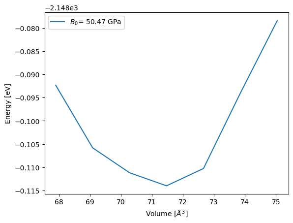
The resulting energies for the different volumes are fitted using a 3rd order polynomial to derive the bulk modulus as second derivative multiplied by the equilibrium volume.

fit_dict = analyse_results_for_energy_volume_curve(
    output_dict={"energy": result_dict},
    task_dict=task_dict,
    fit_type="polynomial",
    fit_order=3,
)

The final energy volume curve plot summarizes the results of this calculation.

plt.plot(fit_dict["volume"], fit_dict["energy"], label="$B_0$= %0.2f GPa" % fit_dict["bulkmodul_eq"])
plt.xlabel("Volume [$\AA^3$]")
plt.ylabel("Energy [eV]")
plt.legend()

<>:2: SyntaxWarning: invalid escape sequence '\A'
<>:2: SyntaxWarning: invalid escape sequence '\A'
/tmp/ipykernel_31059/4024930470.py:2: SyntaxWarning: invalid escape sequence '\A'
  plt.xlabel("Volume [$\AA^3$]")

<matplotlib.legend.Legend at 0x7f507b028ce0>